Day 0: Introduction to Machine Learning

" Machine learning is the science of getting computers to learn without being explicitly programmed "

Today, I explored the fundamentals of Machine Learning, specifically focusing on supervised learning and linear regression. These are notes I took after watching the Machine Learning Specialization course from Coursera offered by Deeplearning.ai and Stanford Online.

Supervised Learning

Supervised learning refers to algorithms that learn x to y or input to output mappings.

The key characteristic of supervised learning is that you give your learning algorithm examples to learn from. That means the correct answers or label y for a given input x

let's take a look at some examples of supervised learning:

Input (x)	Output (y)	Application
email	spam? (0/1)	spam filtering
audio	text transcripts	speech recognition
English	Spanish	machine translation
ad, user info	click? (0/1)	online advertising
image, radar info	position of other cars	self-driving car
image of phone	defect? (0/1)	visual inspection

Regression Model: Linear Regression

Regression is a type of supervised learning that tries to predict a number from infinitely many possible numbers

Linear regression model means fitting a straight line to your data. It's probably the most widely used learning algorithm in the world today.

We'll use the following dataset as an example, where we try to predict the price of a house(y) based on the size of the house in sqft (x)

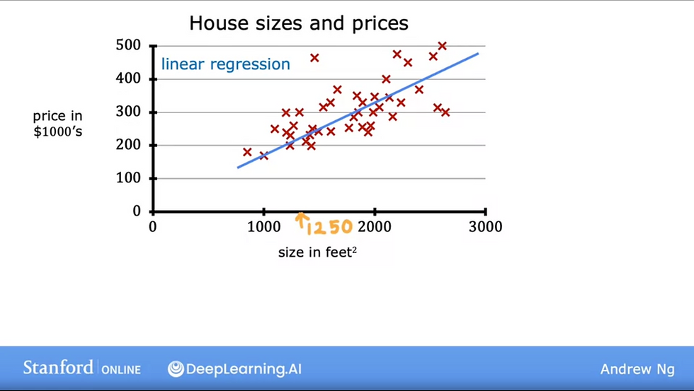
notation: horizontal line represent (x) input features measured in sqft vertical line represent (y) output / target variable red crosses represent each training example

blue straight line represent the regression model

The process of the supervised learning algorithm looks somewhat like this:

1. to train the model, you feed the training set, both the input features (x) and the output target (y) to your learning algorithm.

2. then, your supervised learning algorithm will produce some function (f)

3. the job of f is to take a new input (x) and output a prediction (ŷ) aka y-hat

4. In Machine Learning, the convention is that ŷ is the estimate / prediction for y

5. the function (f) is called the model

When we design a learning algorithm, some of our key questions would include, "How are we going to represent the function f?", or "What's the math formula we're going to use to compute f?"

For now, let's stick with f being a straight line, and our function can be written as:

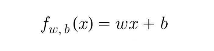
We can write our model function in Python as:

import numpy as np
    
def compute_model_output(x, w, b):
    m = x.shape[0]                # m = number of training examples
    f_wb = np.zeros(m)
    for i in range(m):
        f_wb[i] = w * x[i] + b
    return f_wb

w and b are the parameters of the models. In machine learning, parameters of the model are the variables you can adjust during training to improve the model. They may also be referred to as coefficients or weights

We'll explore the w and b values in the next section, the cost function formula

Cost Function Formula

The cost function will tell us how well the model is doing

To implement linear regression, the first key step is to define a cost function. It will tell us how well the model is doing so that we can try to get it to do better.

We looked at w and b earlier, which are the parameters to our model. let's take a look at what these parameters can do.

• depending on the values you've chosen for w and b, you will get a different function (f), which generates different line on the graph

• you can write f(x) as a shorthand for fw,b(x)

Let's look at 2 examples, with different w and b values, but the same x and y data. This will show us how choosing different w and b values will affect our prediction.

x = np.array([0.0, 1.0,  2.0])
y = np.array([0.0, 0.5, 1])

Example 1 w = 0.5 and b = 0 f(x) = (0.5) x + 0 f(0) = (0.5) (0) + 0 = 0 f(1) = (0.5) (1) + 0 = 0.5 f(2) = (0.5) (2) + 0 = 1

Example 2 w = 0 and b = 1.5 f(x) = (w) (x) + b f(0) = (0) (0) + 1.5 = 1.5 f(1) = (0) (1) + 1.5 = 1.5 f(2) = (0) (2) + 1.5 = 1.5

In regression model, we try to fit our prediction line as close as possible to the actual values. As we can see from the two examples above, when choosing w and b values, one value pair fits our model closer than the other. While the other, example 2, the prediction line is far from our actual values, and will not be a good prediction model.

This is where our cost function comes in, to measure how well a line fits a training data:

• the cost function takes the prediction ŷ and compare it to the target y. This difference is called an error = (ŷ - y). We're measuring how far off to prediction is from target.

• Next, we're going to compute the square of (ŷ-y)

• Since we want to measure the error across the entire training set, and not just one input variable. We will want to compute the average, our function will look like this thus far:

• m is the number of training examples, we will sum the error starting from i=1, all the way up to m (the number of training examples). We will then divide them by m, to get the average.

• Finally, by convention, the cost function that most people use in Machine Learning is divided by '2m'. The extra division by 2 is meant to make some of our later calculations look neater, but the cost function will still work whether we include the division by 2 or not.

• Our cost function now looks like this, we will use the term J(w,b) to refer to the cost function:

• This is also known as the squared error cost function, and it's called that because you're taking the square of these error terms.

• In machine learning, different cost functions may be used, but the squared error cost function by far is the most commonly used one for linear regression and all regression problems, where it gives good results for many applications.

• Just as a reminder as well, ŷ (prediction) is computed through the f(x) function, wx + b

• So, our final cost function will look like this:

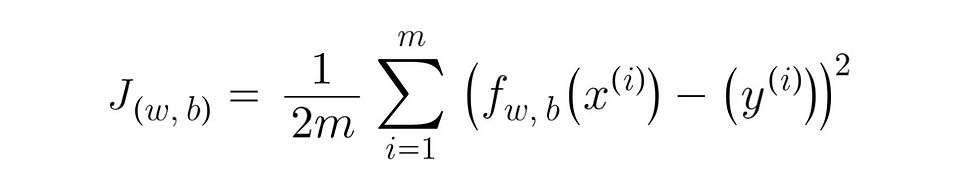
• notation: w and b are parameters of our model m = number of training examples f(x) = the model function to predict our prediction x = input feature y = output variable ŷ = prediction

We can write our cost function J in Python as:

import numpy as np

def compute_cost(x, y, w, b):
    m = x.shape[0]
    cost_sum = 0
    
    for i in range(m):
        f_wb = w * x[i] + b
        cost = (f_wb - y[i]) ** 2
        cost_sum += cost
    
    total_cost = (1 / (2 * m)) * cost_sum
    
    return total_cost

The goal of linear regression is to make J(w,b) or the cost function as small as possible.

We'll explore more about the cost function tomorrow.