Day 3: Gradient descent (part 2)

Gradient Descent

Gradient descent is an algorithm that you can use to find the value of w and b in a more systematic way, which results in the smallest possible of the cost function J(w,b)

What we're going to focus today it to get more understanding about what the learning rate and what the derivative term are doing and why when multiplied together, it results in updates to parameters w and b that makes sense.

tools

import math, copy
import numpy as np
import matplotlib.pyplot as plt
plt.style.use('./deeplearning.mplstyle')
from lab_utils_uni import plt_house_x, plt_contour_wgrad, plt_divergence, plt_gradients

Note: you may need to download some of the libraries needed to run the code in the post, such as lab_utils_uni, which is available on the course's lab

problem statement

let's use the same 2 data points we previously used with our cost function example:

• a house with 1000 sqft sold for $300,000

• a house with 2000 sqft sold for $500,000

# load our data set
x_train = np.array([1.0, 2.0])        # size in 1000 sqft
y_train = np.array([300.0, 500.0])     # price in 1000s of dollar

Compute Cost

This was developed during our Cost Function post, we will be using it again here:

# function to calculate the cost

def compute_cost(x, y, w, b):
    m = x.shape[0]
    cost = 0
    
    for i in range(m):
        f_wb = w * x[i] + b
        cost = cost + (f_wb - y[i]) ** 2
    total_cost = 1 / (2*m) * cost
    
    return total cost

Gradient descent summary

Let's recap the mathematical functions we have seen so far:

• (1) a linear model that predicts the 'f function' f(x):

in linear regression, we utilize input training data to fit the parameters w, b by minimizing a measure of the error between our predictions f(x) and the actual data y. The measure is called the cost function J(w,b)

• (2) In training, you measure the cost over all of our training samples x_i, y_i:

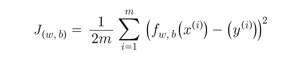
please note that during our python code the sum would start at 'i=0' instead of 'i=1' as Python starts counting from 0, instead of 1, and would end at 'm - 1' instead of 'm'.

• (3) yesterday, we looked at our gradient descent algorithm, which would be described as:

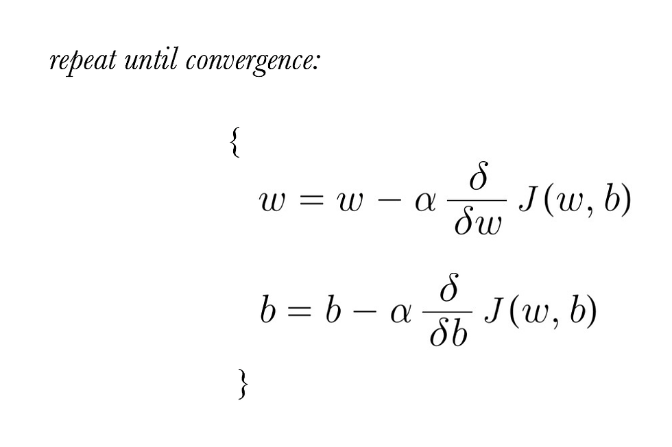
• where, parameters w, b are updated simultaneously, the gradient is defined as:

Implement gradient descent

We will implement gradient descent algorithm for one feature. We will need 3 functions:

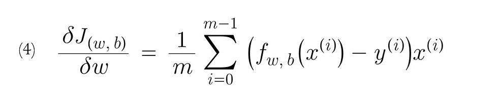
• compute_gradient, implementing equation (4) and (5) above

• compute_cost, implementing equation (2) above (this was already done in our compute cost section above)

• gradient_descent, utilizing compute_gradient and compute_cost

naming conventions:

• the naming of python variables containing partial derivatives will follow this pattern dj_db will be:

• wrt is 'with respect to', as in partial derivative of J(w,b) with respect to b

Compute Gradient

compute_gradient implements (4) and (5) above and returns dj_dw, dj_db

def compute_gradient(x, y, w, b):
    m = x.shape[0]
    dj_dw = 0
    dj_db = 0
    
    for i in range(m):
        f_wb = w * x[i] + b
        dj_dw_i = (f_wb - y[i]) * x[i]
        dj_db_i = (f_wb - y[i])
        dj_db += dj_db_i
        dj_dw += dj_dw_i
    dj_dw = dj_dw / m
    dj_db = dj_db / m
    
    return dj_dw, dj_db

Let's use our compute_gradient function to find and plot some partial derivatives of our cost function relative to one of the parameters w0:

plt_gradients(x_train, y_train, compute_cost, compute_gradient)
plt.show()

• Above, the left plot shows dj_dw or the slope of the cost curve relative to w at three points.

• On the right side, of the plot, the derivative is positive, while on the left in negative. Due to the bowl shape, the derivatives will always lead gradient descent toward the bottom where the gradient is 0.

• The left plot has fixed b=100. Gradient descent will utilize both dj_dw and dj_db to update parameters.

• The quiver plot on the right provides a means of viewing the gradient of both parameters. The arrow sizes reflect the magnitude of the gradient at that point. The direction and slope of the arrow reflects the ratio of dj_dw and dj_db at that point.

Gradient descent

Now that gradients can be computed, gradient_descent, described in equation (3) can be implemented in our function below. We will utilize this function to find optimal values of w and b on the training data.

def gradient_descent(x, y, w_in, b_in, alpha, num_iters, cost_function, gradient_function):

    J_history = []
    p_history = []
    b = b_in
    w = w_in
    
    for i in range(num_iters):
        dj_dw, dj_db = gradient_function(x, y, w, b)
        
        b = b - alpha * dj_db
        w = w - alpha * dj_dw
        
        if i < 100000:
            J_history.append(cost_function(x, y, w, b))
            p_history.append([w, b])
        
        if i%math.ceil(num_iters/10) == 0:
        print(f"Iteration {i:4}: Cost {J_history[-1]:0.2e} ",
              f"dj_dw: {dj_dw: 0.3e}, dj_db: {dj_db:0.3e} ",
              f"w: {w: 0.3e}, b: {b: 0.5e} ")
              
    return w, b, J_history, p_history

Let's run the following code to look at the w, b found by gradient descent using the gradient_descent function we just did:

#initialize parameters
w_init = 0
b_init = 0

# gradient descent settings
iterations = 10000
tmp_alpha = 1.0e-2

# run gradient descent
w_final, b_final, J_hist, p_hist = gradient_descent(x_train, y_train, w_init, b_init, tmp_alpha, iterations, compute_cost, compute_gradient

print(f"(w,b) found by gradient descent: ({w_final: 8.4f}, {b_final: 8.4f})")

Result:

Iteration    0: Cost 7.93e+04  dj_dw: -6.500e+02, dj_db: -4.000e+02   w:  6.500e+00, b: 4.00000e+00
Iteration 1000: Cost 3.41e+00  dj_dw: -3.712e-01, dj_db:  6.007e-01   w:  1.949e+02, b: 1.08228e+02
Iteration 2000: Cost 7.93e-01  dj_dw: -1.789e-01, dj_db:  2.895e-01   w:  1.975e+02, b: 1.03966e+02
Iteration 3000: Cost 1.84e-01  dj_dw: -8.625e-02, dj_db:  1.396e-01   w:  1.988e+02, b: 1.01912e+02
Iteration 4000: Cost 4.28e-02  dj_dw: -4.158e-02, dj_db:  6.727e-02   w:  1.994e+02, b: 1.00922e+02
Iteration 5000: Cost 9.95e-03  dj_dw: -2.004e-02, dj_db:  3.243e-02   w:  1.997e+02, b: 1.00444e+02
Iteration 6000: Cost 2.31e-03  dj_dw: -9.660e-03, dj_db:  1.563e-02   w:  1.999e+02, b: 1.00214e+02
Iteration 7000: Cost 5.37e-04  dj_dw: -4.657e-03, dj_db:  7.535e-03   w:  1.999e+02, b: 1.00103e+02
Iteration 8000: Cost 1.25e-04  dj_dw: -2.245e-03, dj_db:  3.632e-03   w:  2.000e+02, b: 1.00050e+02
Iteration 9000: Cost 2.90e-05  dj_dw: -1.082e-03, dj_db:  1.751e-03   w:  2.000e+02, b: 1.00024e+02
(w,b) found by gradient descent: (199.9929,100.0116)

Let's take a moment and note some characteristics of the gradient descent process above:

• the cost starts large and rapidly declines as described before

• the partial derivatives, dj_dw, and dj_db also get smaller, rapidly at first and then more slowly. the process near the 'bottom of the bowl' progress slower due to the smaller value of the derivative at that point

• progress slows, although the learning rate (alpha) remains fixed.

Cost vs iterations of gradient descent

A plot of cost vs iterations is a useful measure of progress in gradient descent. Cost should always decrease in successful runs. The change in cost is so rapid initially, it is useful to plot the initial descent on a different scale than the final descent. In the plots below, note the scale of cost on the axes and the iteration step

Predictions

Now that we have discovered the optimal values for the parameters w and b, we can use the model to predict housing values based on our learned parameters:

print(f"1000 sqft house prediction {w_final*1.0 + b_final:0.1f} Thousand dollars")
print(f"1200 sqft house prediction {w_final*1.2 + b_final:0.1f} Thousand dollars")
print(f"2000 sqft house prediction {w_final*2.0 + b_final:0.1f} Thousand dollars")

Result:

1000 sqft house prediction 300.0 Thousand dollars
1200 sqft house prediction 340.0 Thousand dollars
2000 sqft house prediction 500.0 Thousand dollars

Plotting

We can show the progress of gradient descent during its execution by plotting the cost over iterations on a contour plot of the cost(w, b).

fig, ax = plt.subplots(1,1, figsize=(12, 6))
plt_contour_wgrad(x_train, y_train, p_hist, ax)

The contour plot above shows the cost value J(w,b) over a range of w and b. Cost levels are represented by rings. the red arrows is the path of gradient descent. The path makes steady progress towards its goal and the initials steps are much larger than the steps near the goal.

Tomorrow: let's take a deeper look at our learning rate (alpha)