Day 5: summary of introduction to machine learning
- eyereece
- Jun 22, 2023
- 4 min read

Machine learning is the science of getting computers to learn without being explicitly programmed
Supervised learning
Supervised learning refers to algorithms that learn x to y or input to output mappings
the key characteristic of supervised learning is that you give your learning algorithms examples to learn from, which means the correct answers or 'label y' for a given 'input x'
By seeing correct pairs of input x and desired output label y, the learning algorithm eventually learns to take the input alone without the output label and gives a reasonably accurate prediction or guess of the output
Some examples include, but are not limited to, spam filtering, speech recognition, machine translation, online ads, self-driving car, etc
2 main algorithms used in supervised learning:
regression: predict a number from infinitely many possible outputs
classification: predict categories from a smaller number of possible outputs
Unsupervised learning
In unsupervised learning algorithm, we give a dataset to the machine and does not give any labels to the data. Instead, it will cluster those data into separate categories, and find some structure in it
This is called clustering algorithm, when there's separate cluster groups and place unlabeled data into different clusters
An example of this is Google news, when you look up a phrase it will also show related articles mentioning panda as well. So, it looks at hundreds or thousands of news articles on the internet, and group related stories together.
Regression model (linear regression)
linear regression model means fitting a straight line to your data.
In the example below, we try to predict the price of a house based on the size of the house.
The red cross is the actual output value y, and the blue straight line is model function/prediction line
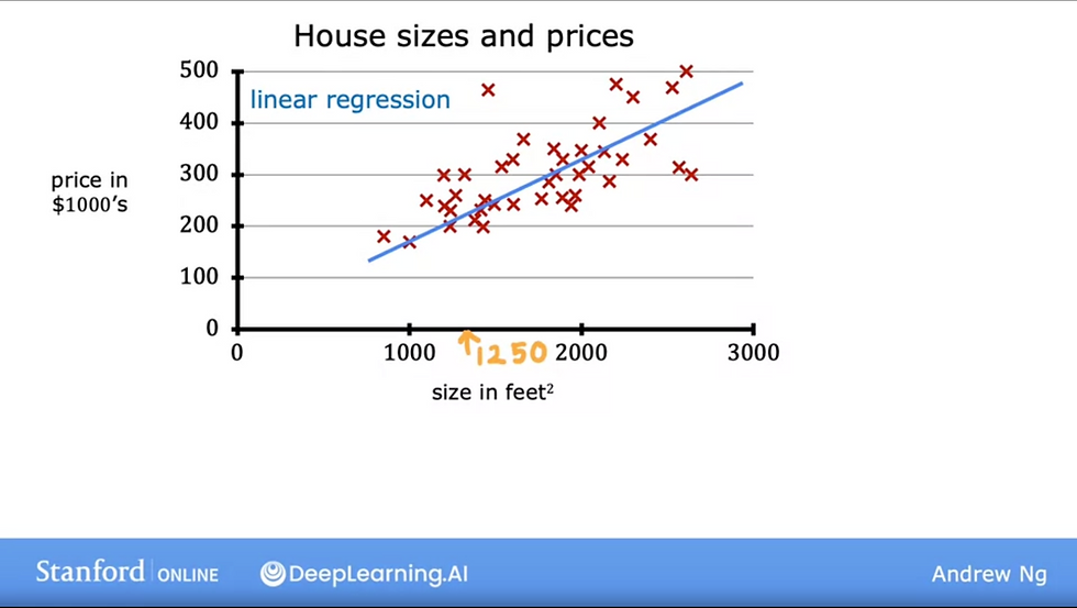
The size of the the house is the input feature, notated as x
the actual price of the house given x is the output variable, notated as y
m = the number of training examples
The process of the supervised learning algorithm looks somewhat like this:
to train the model, you feed the training set, both the input features (x) and the output target (y) to your learning algorithm.
then, your supervised learning algorithm will produce some function (f)
the job of f is to take a new input (x) and output a prediction (ŷ) aka y-hat
In Machine Learning, the convention is that ŷ is the estimate / prediction for y
the function (f) is called the model
When we design a learning algorithm, some of our key questions would include, "How are we going to represent the function f?", or "What's the math formula we're going to use to compute f?"
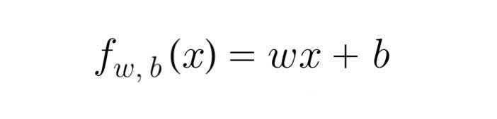
For now, let's stick with f being a straight line, and our function can be written as, we can refer to fw,b(x) as f(x):
The code for the model function is:
import numpy as np

def compute_model_output(x, w, b):
    m = x.shape[0]
    f_wb = np.zeros(m)
    for i in range(m):
        f_wb[i] = w * x[i] + b

    return f_wb
The cost function
In order to implement linear regression, the first key step is to define a cost function
the cost function will tell us how well the model is doing so that we can try to get it to do better
the model we're going to use to fit the training set is the linear function:
w and b are the parameters of the model, weight and bias
In machine learning, parameters of the model are the variables you can adjust during training in order to improve the model.
Sometimes, the parameters w and b may also be referred to as coefficients or weights.
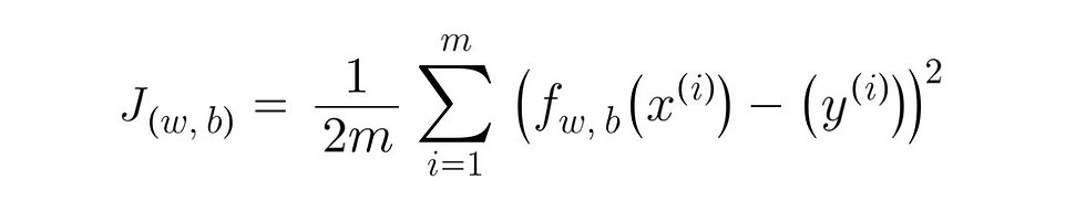
In this course, the cost function is referred to as J, and the algorithm of the cost function is:
the code for the cost function in Python:
import numpy as np

def compute_cost(x, y, w, b):
    m = x.shape[0]
    cost_sum = 0

    for i in range(m):
        f_wb = w * x[i] + b
        cost = (f_wb - y[i]) ** 2
        cost_sum += cost
    total_cost = (1/(2*m)) * cost_sum

    return total_cost
for linear regression, if the selected parameters w and b causes the cost function J to be very close to 0, we can conclude that the selected values of the parameters cause the algorithm to fit the training set very well.
The goal of the cost function J is to be as close to 0 as possible.
gradient descent
Gradient descent is an algorithm we can use to find the values of w and b in a more systematic way, which results in the smallest possible cost of J
An overview of what gradient descent does is, if you have a cost function J that you want to minimize to a minimum, with gradient descent, you'll keep changing the parameter w and b by a little bit every time to reduce the cost function J, until J settles at or near a minimum
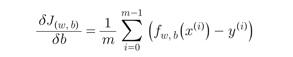
The algorithm for gradient descent:
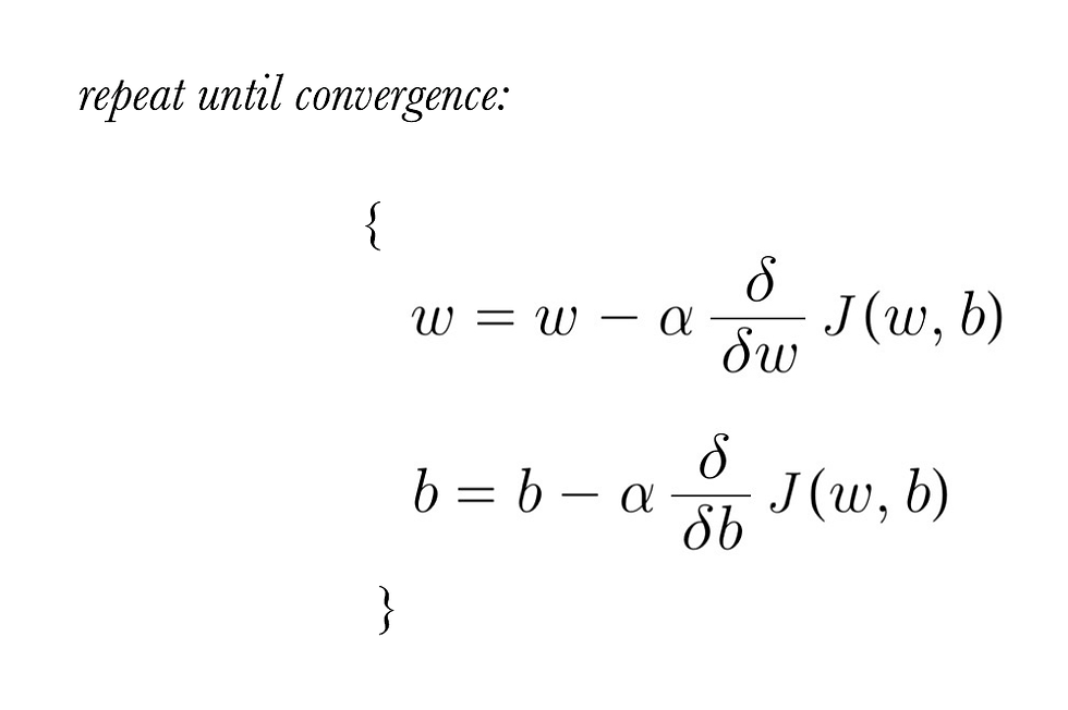
where:
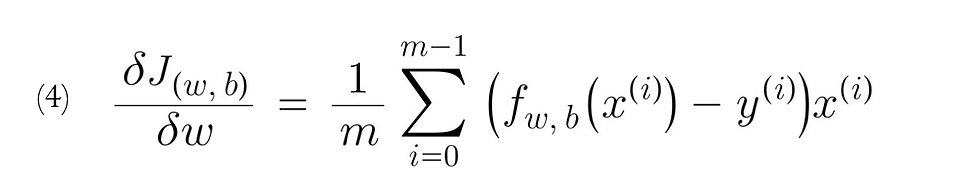
Note: please ignore the number '(4)' in the derivative term for 'dw', it is not a part of the function and the image was used for notation purposes in previous post
the code for implementing gradient descent in Python, we'll first start by creating a function to find the values of dj_dw, and dj_db
def compute_gradient(x, y, w, b):
    m = x.shape[0]
    dj_dw = 0
    dj_db = 0

    for i in range(m):
        f_wb = w * x[i] + b
        dj_dw_i = (f_wb - y[i]) * x[i]
        dj_db_i = f_wb - y[i]
        dj_db += dj_db_i
        dj_dw += dj_dw_i

    dj_dw = dj_dw/m
    dj_db = dj_db/m

    return dj_dw, dj_db
we'll then run gradient descent with the code below, using the cost function (compute_cost) we created earlier and gradient function (compute_gradient):
def gradient_descent(x, y, w_in, b_in, alpha, num_iters, cost_function, gradient_function):
      J_history =[]
      p_history =[]
      b = b_in
      w = w_in

      for i inrange(num_iters):
            dj_dw, dj_db = gradient_function(x, y, w, b)

            b = b - alpha * dj_db
            w = w - alpha * dj_dw

            if i <100000:
                  J_history.append(cost_function(x, y, w, b))
                  p_history.append([w, b])
            if i%math.ceil(num_iters/10)==0:
                  print(f"Iteration {i:4}: Cost {J_history[-1]:0.2e} ",
                  f"dj_dw: {dj_dw: 0.3e}, dj_db: {dj_db:0.3e} ",
                  f"w: {w: 0.3e}, b: {b: 0.5e} ")

       return w, b, J_history, p_history
the learning rate (alpha) is a positive number between 0 - 1
it basically controls how big of a step the function takes downhill to reach a minimum.
the gradient process of taking small steps until it reach a global minimum is called batch gradient descent
Comments