Day 8: Feature Scaling and learning rate

Feature Scaling

Feature scaling is a technique that will enable gradient descent to run faster.

let's start by taking a look at the relationship between the size of a feature and the size of it's associated parameter

price-prediction = W1*X1 + W2*X2 + b

notation:

X1 = size = 300 - 2000 sqft

X2 = number of bedrooms = 0 - 5

In this example, House: X1 = 2000, X2 = 5, price = $500k

What do you think would be the appropriate parameters W (W1 and W2) and b?

Let's look at a couple examples:

Example 1

W1 = 50, W2 = 0.1, b = 50

price-prediction = 50*2000 + 0.1*5 + 50 = 100k + 0.5 + 50k

price-prediction = $100,050.5

price-prediction is off as the price is way cheaper than the actual price of $500,000

Example 2

W1 = 0.1, W2 = 50, b = 50

price-prediction = 0.1*2000 + 50*5 + 50 = 200k + 250k + 50k

price-prediction = $500,000

price-prediction in this scenario is more accurate

You may notice from the examples above that when possible range of values of a feature is large, for instance the size in sqft which goes all the way up to 2000, it's more likely a good model will learn to choose a relatively small parameter value.

likewise, when the possible values of the feature are small, the number of bedrooms, then a reasonable value for its parameters will be relatively large.

so, how does this affect gradient descent?

Let's say you're trying to run gradient descent with 2 features that has very large range difference. For example, X1 = 0 - 1, X2 = 10 - 100.

If you were to use your data "as-is" in this situation, contour plot may be shaped more like a skinny oval as opposed to a circle, and because of that, gradient descent may end up bouncing back and forth for a long time, before it finally reach a minimum.

In these situations, it's usually a good idea to scale the features, which means performing some transformation of your training data so that X1 and X2 might range from 0-1

The key point is that the re-scaled X1 and X2 are both now taking comparable ranges of values to each other.

How to scale features?

There are a few different ways to scale features:

• divide by max

• mean normalization

• z-score normalization

divide by max

let's take a look at an example:

x1 = 300 - 2000 # x1 is a value between 300 to 2000

300 ≤ x1 ≤ 2000

x1-scaled = x1 / 2000 # x1 divided by maximum value (in this case 2000)

0.15 ≤ x1-scaled ≤ 1 # x1 scaled is now a value between 0.15 to 1

x2 = 0 - 5 # x2 is a value between 0 to 5

0 ≤ x1 ≤ 5

x2-scaled = x2 / 5 # x2 divided by maximum value (in this case 5)

0 ≤ x2-scaled ≤ 1

mean normalization

Another way to feature scale is to implement mean-normalization.

In mean normalization, you start with the original features, and then, you re-scale them so that both of them are centered around zero, where they previously only had values greater than zero, they now have values ranging from -1 to 1

the formula for mean normalization:

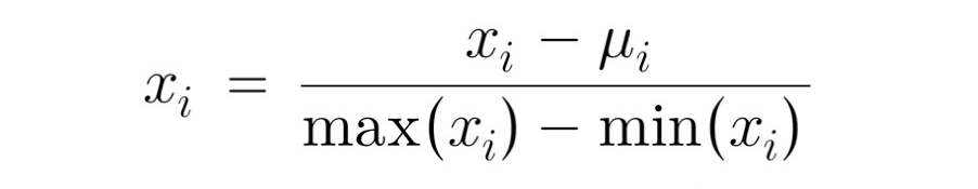
μ = mean

An example:

300 ≤ x1 ≤ 2000

x1-scaled = (x1 - μ1) / (2000 - 3000)

-0.18 ≤ x1-scaled ≤ 0.82

0 ≤ x2 ≤ 5

x2-scaled = (x2 - μ2) / (5 - 0)

-0.46 ≤ x2-scaled ≤ 0.54

z-score normalization

z-score normalization is another re-scaling method.

to implement z-score normalization, you'll need calculate standard-deviation(σ) of each feature

The formula for z-score normalization:

An example:

300 ≤ x1 ≤ 300

x1-scaled = (x1 - μ1) / σ1

-0.67 ≤ x1-scaled ≤ 3.1

z-score normalization: implementation

After z-score normalization, all features will have a mean of 0 and a standard deviation of 1. Using the above formula, let's code this:

# import libraries
import numpy as np

def z_score_normalize_features(X):
    # find the mean of each column/feature
    mu = np.mean(X, axis=0)
    # find the standard deviation of each column/feature
    sigma = np.std(X, axis=0)
    # element-wise, subtract mu for that column from each example, divide by std for that column
    X_norm = (X - mu) / sigma
    
    return (X_norm, mu, sigma)

please note that you may use the Scikit-learn library to implement feature scaling without coding this with the NumPy library shown here.

Take a look at the distribution of of features before, during, after normalization:

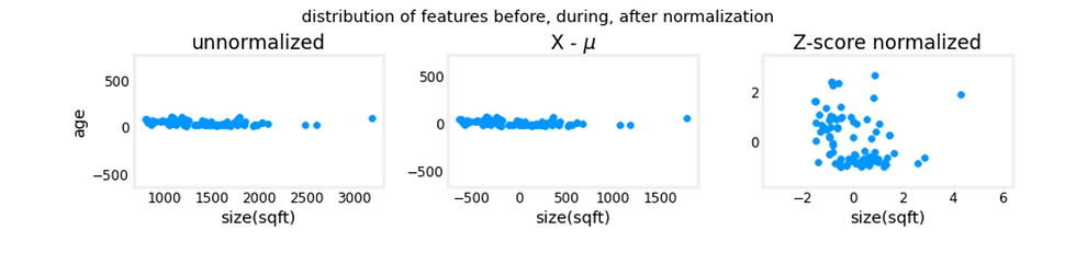
The plot above shows the relationship between two of a training set parameters, "age" on the vertical axis, and "size(sqft)" on the horizontal axis.

Rule of thumb for feature scaling

aim for about:

- 1 ≤ Xj ≤ 1 # for each feature Xj

-3 ≤ Xj ≤ 3 # acceptable ranges

-0.3 ≤ Xj ≤ 0.3 # acceptable ranges

0 ≤ x1 ≤ 3 # okay, no rescaling

-2 ≤ x2 ≤ 0.5 # okay, no rescaling

-100 ≤ x3 ≤ 100 # too large, re-scale

-0.001 ≤ x4 ≤ 0.001 # too small, re-scale

98.6 ≤ x5 ≤ 105 # too large, re-scale

when in doubt, re-scale

Checking gradient descent for convergence

recall that the objective of gradient descent is to reach the minimum of cost-function J.

J(w, b) should decrease after every iteration. Number of iteration varies, could be as little as 30, to as large as 100,000

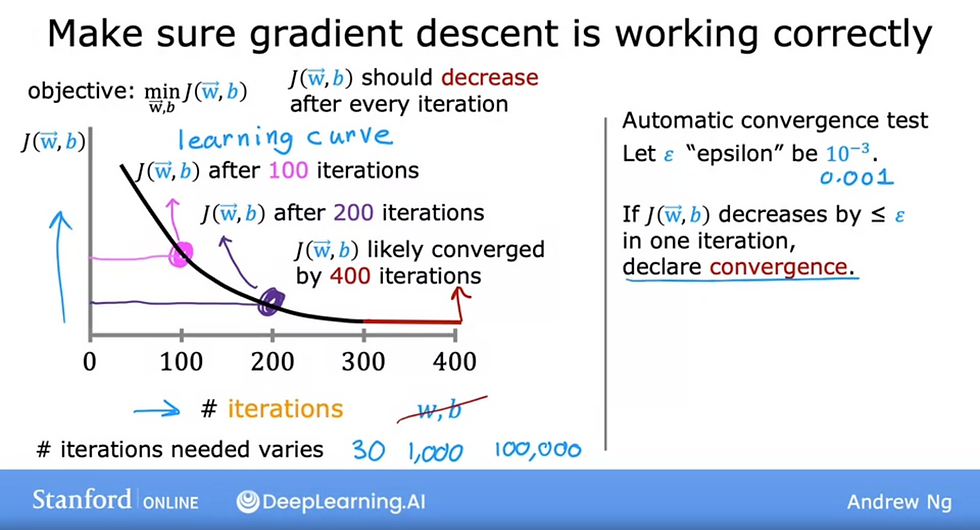
Take a look at the learning curve graph above, once the line has flattened (the red line of the curve), J(w,b) most likely has converged.

Another way to see if gradient descent have reached a minimum is through the 'Automatic convergence test'

let ε "epsilon" be 0.001

if J(w, b) decreases by ≤ ε in one iteration, declare convergence

it's usually pretty difficult to choose the right threshold epsilon and may be easier to look at the learning curve graph

Choose the learning rate (α)

Your learning algorithm will run much better with an appropriate choice of learning. recall that if the learning rate is too small, it will take forever to converge, and if it is too large, it may never converge.

Concretely, if when you plot the cost for the number of iterations, notice that the cost sometimes go up and down, that could be a sign of either a large learning rate or a bug in the code.

It's recommended to start with a very small learning rate to make sure there's no bug in the code. If the cost slowly decreases (with no increment), then we know that there's no bug and we can slowly build up the value of the learning rate

You may start with '0.001', and increase the learning rate by 3x to '0.003', and again, and so forth, with each value of alpha roughly 3x bigger than the previous value.

After trying these ranges, try to pick the largest possible learning rate, or something slightly smaller than the large value that we found.