Introduction
The objective of this project is to develop a model to detect and identify fashion objects in images and provide bounding box coordinates for each identified fashion class.
This project utilizes an object detection model trained on fashion categories, specifically the YOLOv5 network from Ultralytics. The jupyter notebooks for this project is available on my GitHub repo here: https://github.com/eyereece/yolo-object-detection-fashion The repo contains the following notebooks (completed in the following order):
data_preparation
yolo_training
yolo_prediction
Additionally, it also contains a data.yaml that follows the folder structure outlined below for training.
Data Preparation
The dataset I used for this project is from a public dataset for the paper "Bootstrapping Complete the Look at Pinterest" available here
For this project I used the raw_train.tsv file which consists of the following information:
image signature
normalized x coordinate
normalized y coordinate
normalized width
normalized height
label
The images in the dataset are represented by a signature and the corresponding image URL is obtained through the following code:
def convert_to_url(signature):
    prefix = 'http://i.pinimg.com/400x/%s/%s/%s/%s.jpg'
    return prefix % (signature[0:2], signature[2:4], signature[4:6], signature)
Data Pre-Processing
To collect the images and their respective bounding box information, I did the following:
Cleaned and transformed the dataframe with pandas: extracted and organized its column names, removed empty strings
To obtain a more balanced dataset across categories, I set the script to collect 1000 images per category, resulting in a total of 15,657 objects and 9,235 images.
As these images are obtained from the web, many of the images are corrupt, I used an ImageMagick mogrify script to fix them.
Calculated normalized center x and center y for the bounding box coordinates.
Mapped class labels to its respective integer values for ground truth labels for model training
Created a .txt file for each image containing the filename, classId, center_x, center_y, w, and h for model training
Create a data.yaml file for model training
Organized the images and its respective information per the data.yaml specification created.
The images and its respective information (stored in a .txt format) is stored in the following folder structure:
data_images
|
|-----train
|     |----- 001.jpg
|     |        |
|     |
|     |----- 001.txt
|     |        |
|     |
|
|-----test
|     |----- 1001.jpg
|     |        |
|     |
|     |----- 1001.txt
|     |        |
|     |
Bounding Box Formula
As noted in the data information above, the normalized x and y coordinates were given. To train the YOLOv5 model, normalized center_x and center_y is needed.
The following image shows the coordinates of bounding boxes:
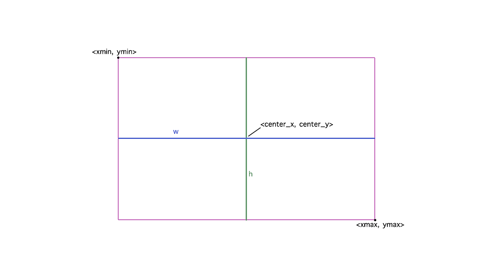
To calculate center_x and center_w, I first need to obtain the xmin, ymin, xmax, and ymax, which can be obtained through the following (code made available from the public dataset's GitHub page):
im_w, im_h = image.size
box = (x * im_w, y * im_h, (x + width) * im_w, (y + height) * im_h)
To convert them to center_x and center_y, I used the following formula:


Data Exploration
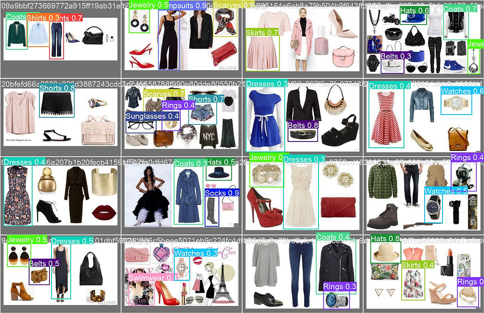
The following images show collages of images in the dataset along with their bounding boxes and class labels:
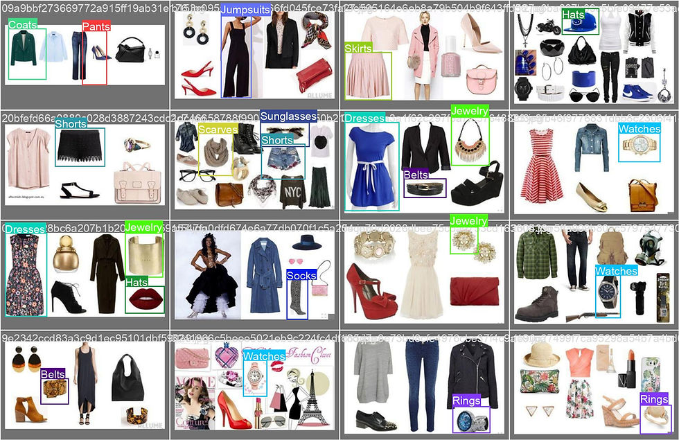
Most of the bounding boxes are labeled correctly; however, a few bounding box coordinates are not precisely placed, as seen in the top left image containing a 'pants' instance.
The most noticeable issue arising from training with the dataset is that many fashion objects or instances in each image are not labeled. This may result in low recall in the model, leading to the detection of more false negatives.
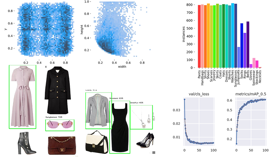
Let's take a look at some of the plots related to the labels in the dataset:
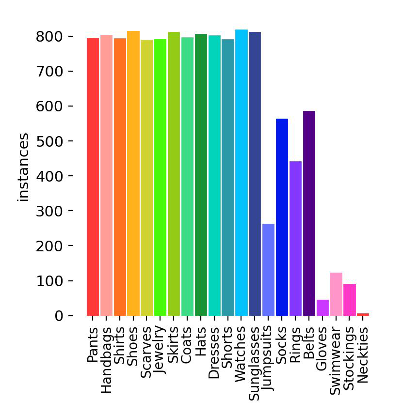
Most of the labels are evenly distributed as per the specifications set during data preparation, but some labels are still under-represented, such as jumpsuits, socks, rings, and most of the class labels on the right side of the plot.
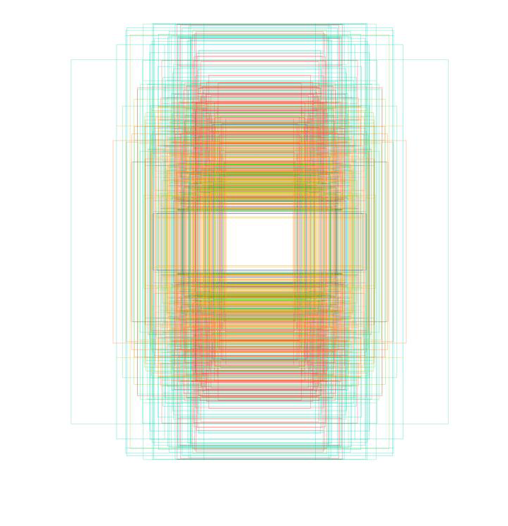
The grid plot above visually represents instances of each class, delineated with colors corresponding to their respective classes. Notably, the majority of instances in the dataset exhibit a greater height compared to their width.
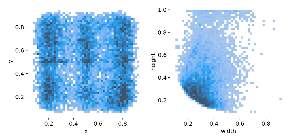
The above plot presents a histogram illustrating the distribution of x, y, width (w), and height (h) coordinates within the dataset:
The left plot displays a Seaborn histogram of x and y coordinates from the dataset, with values ranging from 0 to 1 on both axes. The varying shades of blue represent the concentration of bounding box positions. Darker shades indicate higher concentration, suggesting that, in general, the instances are evenly distributed across the axes, with some localized areas of increased concentration. The rectangular shape of the histogram implies a consistent distribution of x-coordinates in the dataset.
The right plot displays a Seaborn histogram of normalized width and height values of the bounding boxes, it offers insights into the prevalent sizes and proportions of bounding boxes in the dataset. The darker hue can be observed in the bottom-left area, particularly in the range of 0.2 to 0.4 on both the width (w) and height (h) axes, suggesting a concentration of bounding box sizes within this specific region. On the height axis, there is a notable concentration between 0.1 and 0.3, while the width axis shows more concentration in the range of 0.1 to 0.4. The height axis shows a broader distribution with light blue hues spanning from 0 to 1.
Model Configuration, Baseline, and Benchmark
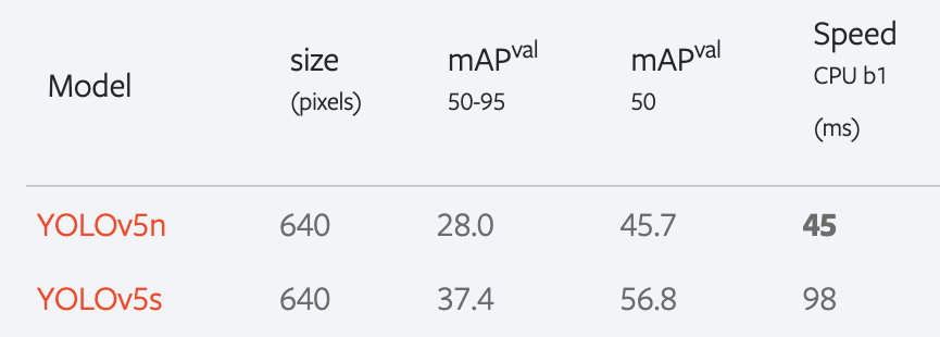
For this project, I used the pretrained YOLOv5 model by Ultralytics, training it for 100 epochs on a T4 GPU within the Google Colab environment. The baseline for this project is established by the performance of the pretrained model on COCO dataset, which is summarized in the following results:
Additionally, an existing detection model, trained on an expanded size of the same dataset and a different model architecture, demonstrates the following result:
mAP | Precision | Recall |
77.2 | 76.0 | 82.4 |
The displayed results are sourced from the original paper, where the dataset was acquired, available here. The model was trained on 251,000 training images using a Faster-RCNN architecture.
Finally, the YOLO model trained for this project exhibits the following performance results:
mAP | Precision | Recall |
60.9 | 54.8 | 64.8 |
The pretrained YOLOv5 model established a baseline with a mAP score of 56.8, whereas the Faster-RCNN model, trained on an expanded dataset, achieved a mAP score of 77.2.
The YOLOv5 model, fine-tuned for this project, attained a score of 60.9, indicating a +4.1 improvement over the baseline.
While the model has shown improvement over the baseline, there is still room for improvement, particularly when compared to the Faster-RCNN architecture used in the expanded dataset. In the following sections, I will delve into my analysis, evaluation, and recommendations for refining the model. Additionally, I will provide an overview of the use case for this model, offering a preview of its application in my forthcoming project.
Model Analysis and Evaluation
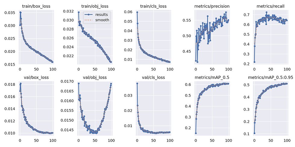
Three loss functions were used to measure the performance of the model: box (CIoU), Objectness (BCE), and Classes Loss (BCE).
Box loss, calculated with Complete Intersection over Union, measures the error in localizing the object within the grid cell.
Objectness loss, calculated with Binary Cross Entropy, calculates the error in detecting whether an object is present in a particular grid cell.
Classes Loss, calculated with Binary Cross Entropy, indicates which object class it belongs to.
From the plots above, all three losses on the training set show continuous improvement throughout the epochs, while validation class loss stabilizes around the midway point, and validation objectness loss starts to degrade from epoch 50 onwards. This may indicate that the model is overfitting to the training set when trying to identify whether an object is present or not.
mAP (mean average precision) shows continual improvement up to epoch 50, after which it plateaus for the remainder of the training. Let's take a look at the following table to see which class is bringing down the mAP:
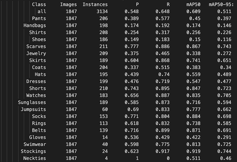
Based on the table above, the mAP50 overall is 0.609. The class categories below that overall score are:
Pants
Handbags
Shirts
Shoes
Jewelry
Coats
Hats
Dresses
Gloves
Neckties
The lower performance doesn't appear to be solely attributed to the number of instances in certain classes. Categories like Jumpsuits, Stockings, Socks, Rings, etc., exhibit higher mAP scores despite having a low number of instances.
Upon closer inspection of classes with low mAP scores, it becomes evident that these classes encompass a significant level of variability. For instance, the Shirts category includes various types such as long sleeve, short sleeve, sweaters, tank tops, etc., and a similar variability is observed in the Jewelry category, which encompasses necklaces, bangles, bracelets, and more.
Examining both the Precision and Recall columns reveals that certain classes encounter notable performance challenges. Classes such as handbags, shirts, shoes, and jewelry exhibit low recall, indicating the model's difficulty in capturing all relevant instances of these categories. Moreover, these same classes demonstrate low precision, emphasizing challenges in accurately identifying and correctly classifying instances.
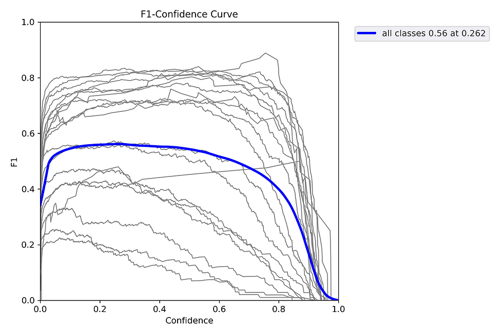
Reviewing the F1-Confidence curve highlights a dip in confidence scores beyond the critical threshold of 0.262. To optimize model performance during inference, it is recommended to set the confidence threshold at or below this value.
The current model from this training achieves the following result:
mAP | Precision | Recall |
60.9 | 54.8 | 64.8 |
Model Results
Let's take a look at a few sample results from the current model:
Image with ground truth labels:
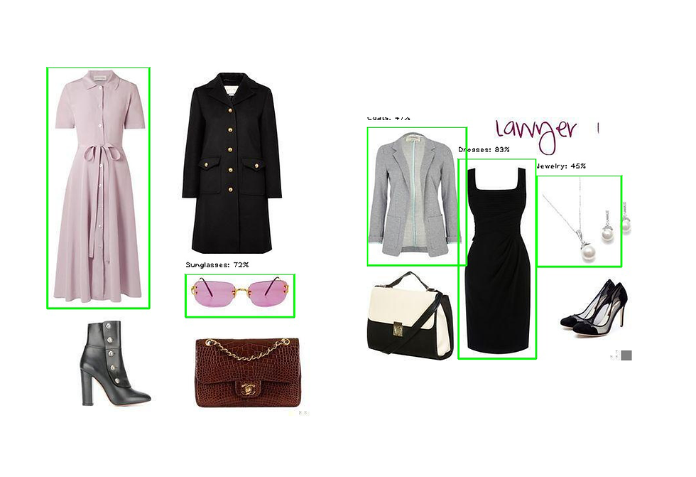
Image with predicted labels:
Looking at the samples above between the images with ground truth labels vs predicted labels, it looks like the model is able to correctly predict many of the objects and even predict objects that did not have ground truth labels on it.
A few other sample results:
Let's now take a look at a real-time demo of the model:

While observing the real-time demo, it is evident that predictions intermittently appear and disappear for the same object as the screen moves through the frames. This behavior could be attributed to the model's low confidence in its predictions for the identified object.
Recommendations for Improvement
Increase Dataset for Underperforming Classes
As highlighted above in the analysis and evaluation section, certain classes consistently exhibit lower scores across all three metrics. This observed trend cannot be solely attributed to a low number of instances in the dataset; upon closer look, these classes demonstrate increased variability in terms of visual attributes.
While acknowledging that the variability within individual classes may contribute to challenges in model generalization, it is imperative to weigh the practical considerations of allocating time and resources to manually curate a more balanced dataset for these classes. Evaluating the tradeoff between the effort required for a curated dataset and the potential model performance gains is crucial.
Alternatively, augmenting the dataset for underperforming classes by introducing randomized samples could enhance model generalization without an extensive manual curation process. This approach warrants consideration, especially when faced with constraints on time and resources. Additionally, the model's performance stagnated on the validation set halfway through training, as evidenced by the three loss metrics discussed in the previous section. This suggests potential overfitting to the training set, indicating a potential for improvement with an expanded dataset.
Add Background Images
To address low precision, often associated with False Positives (incorrect class predictions or predictions in the absence of an object), I would consider incorporating background images (images with no object present), representing 1% to 5% of the total dataset. This measure aims to mitigate the occurrence of false positives.
Label Consistency and Accuracy
As noted above in the analysis and evaluation section, there are a number of unlabeled object instances in images. This may be attributed to the data collection method outlined in the data preparation section. Specifically, the process of collecting 1000 images per class focused on individual instances, which could potentially result in unlabeled instances in images and contribute to the low recall metric. To address this issue, I recommend implementing a script to collect the remaining instances associated with the images currently present in the dataset, ensuring comprehensive labeling of all instances.
Model Use Case (My Next Project Preview)
In the introduction, I mentioned that the the purpose of this project is to develop a model to detect and identify fashion objects in images, but didn't mention my use case for this model once it's able to detect fashion objects, which is to recommend outfits based on the detected fashion items.
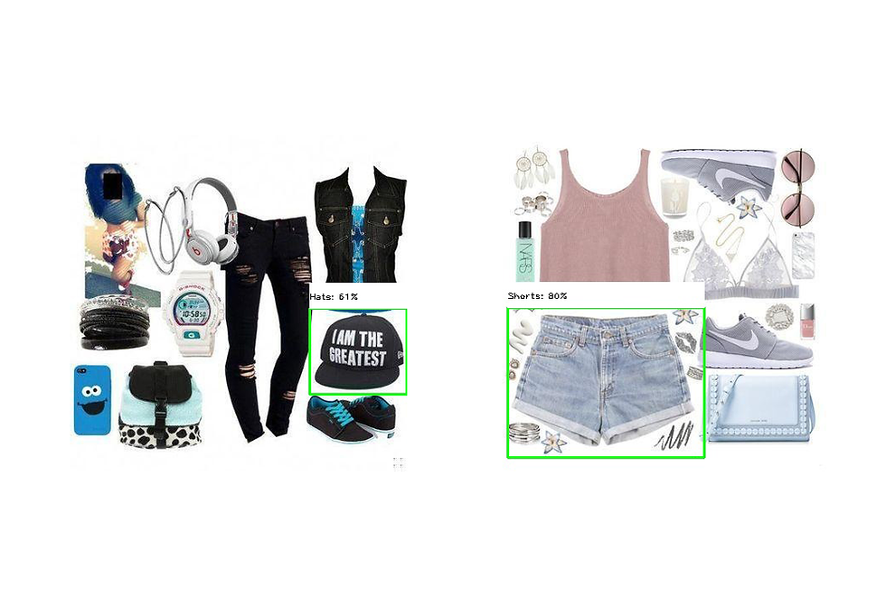
Let's take a look at an example of it in action:
In the gif image above, the model takes an image, detect fashion objects, and display them, it then takes the detected objects and recommends a similar outfit based on the detected objects.
The model essentially takes in an image, detects fashion objects, and crops them into individual images before sending it further for recommendation:
I intend to use this object detection model in my upcoming project, which is currently in progress and showing promising results. I plan to share more details about the project soon. Previously, I have completed a project on similarity search based on visual attributes, and the upcoming project will build upon the concepts outlined in that work. You can find more information about the previous project here
can you please provide me the trained model?
if yes then email me at muheedk999@gmail.com, i am using it as reference model for my fyp.